Our guide below will show you how to apply this formatting to your date to achieve your desired result. You can read our guide on how to see formatting in Excel if you would like to check the current format that is applied to some of the cells in your worksheet.
How to Format for “Year Only” in Excel 2013
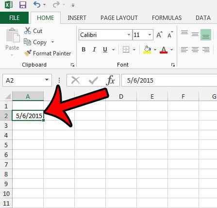
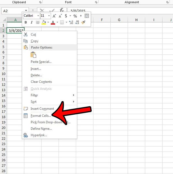
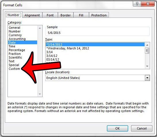
The steps in this article will assume that you have a date in a cell, or group of cells, and that you only want to display the year from that date. The full date will still be stored as the value in the cell, but only the year will be shown. Here is how to only display the year of a date in Excel 2013 – You can see these steps below, but with pictures – Step 1: Open the spreadsheet in Excel 2013. Step 2: Select the cell, or group of cells, containing the dates that you wish to format to only show the year. Step 3: Right-click one of the selected cells, then click the Format Cells option. Step 4: Click Custom in the Category column at the left side of the window. Step 5: Enter yyy into the Type field at the center of the window, then click the OK button to apply your changes. Note that you can also use the formula =YEAR(XX) where XX is the cell containing the date whose year you wish to display. Does your worksheet have a lot of formatting that you need to remove, and you would prefer to simply remove all of it at once? Learn how to clear all cell formatting in Excel with just a few short steps. After receiving his Bachelor’s and Master’s degrees in Computer Science he spent several years working in IT management for small businesses. However, he now works full time writing content online and creating websites. His main writing topics include iPhones, Microsoft Office, Google Apps, Android, and Photoshop, but he has also written about many other tech topics as well. Read his full bio here.
You may opt out at any time. Read our Privacy Policy


